
Azure Sentinel pricing model is driven by the amount of data ingested for security analytics that is stored in the related Log Analytics workspace. Given the costs of the cloud resources, it is important to be able to estimate future logs space consumption and consider any budget-related implications.
Basing the analysis on the past data, a script can be built to determine the trend of the daily log space consumption and then, estimate a log space usage for a future date. It’s worth mentioning that data retention for Sentinel is free for the first 90 days. For longer retention periods, Azure Monitor Log Analytics data retention pricing applies.
The script below uses the consumption data in the Usage table to build a time series array of daily log consumption for the past 90 days.
//define a time range variable for the ingested data (last 90 days)
let timeRange = 90d;
//time in the future for which log usage is to be estimated (in 30 days)
let projectionDays = 30;
//query Usage table
Usage
//filter by selected time range
| where TimeGenerated > ago(timeRange)
//create an array of values for daily log consumption over selected time range
| make-series logConsumption = sum(Quantity) default = 0
on TimeGenerated in range (ago(timeRange) , ago(1d), 1d)
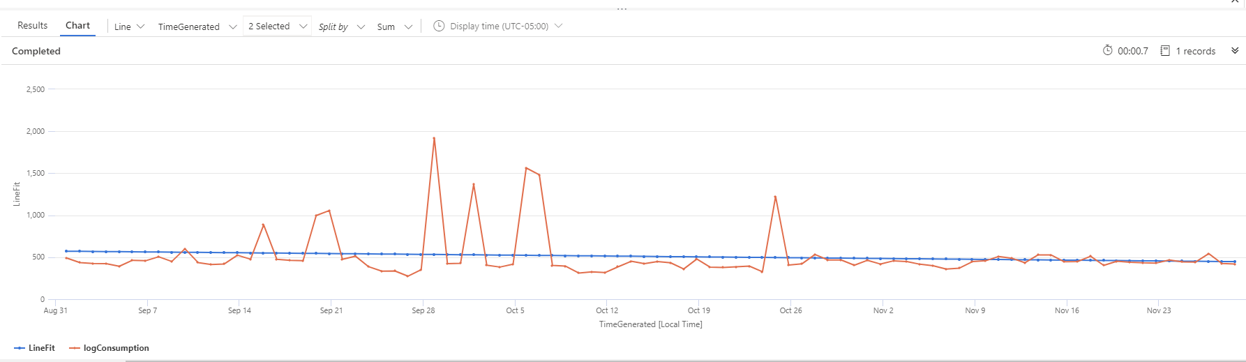
Using KQL’s series_fit_line() command, the best fit line for the series of the daily log consumption values is determined. The LineFit values array represents in this case the log usage trend:
//apply liniar regression to the logConsumption array to determine the values of Slope, Interception, and LineFit
| extend (RSquare,Slope,Variance,RVariance,Interception,LineFit) = series_fit_line(logConsumption)

For a more comprehensive understanding of the output of series_fit_line() command, the trend line and the actual log consumption values can be visualized by rendering a time chart:
To determine the estimated value of the log consumption in 30 days, the script concludes with the below:
//convert the time range to a scalar value
| extend numberOfDaysUsed = timeRange/1d
//calculate estimated log usage on the date 30 days from now
| extend estUsage = Slope*(numberOfDaysUsed + projectionDays) + Interception
//filter to estimated log usage value
| project estUsage

Here, the log space usage on the date 30 days in the future from the current date is 406.178 MB. The value indicates that a move from the current pay-as-you-go pricing model will not be needed.
Download script from GitHub
Final script:
//define a time range variable for the ingested data (last 90 days)
let timeRange = 90d;
//time in the future for which log usage is to be estimated (in 30 days)
let projectionDays = 30;
//query Usage table
Usage
//filter by selected time range
| where TimeGenerated > ago(timeRange)
//create an array of values for daily log consumption over selected time range
| make-series logConsumption = sum(Quantity) default = 0
on TimeGenerated in range (ago(timeRange) , ago(1d), 1d)
//apply linear regression to the logConsumption array to determine parameters like Slope, Interception, LineFit
| extend (RSquare,Slope,Variance,RVariance,Interception,LineFit) = series_fit_line(logConsumption)
//convert the time range to a scalar value
| extend numberOfDaysUsed = timeRange/1d
//calculate estimated log usage on the date 30 days from now
| extend estUsage = Slope*(numberOfDaysUsed + projectionDays) + Interception
//filter to estimated log usage value
| project estUsage
//End of script
Returning to the previous time chart, some spikes in the past log consumption data are observed. In this case, a better option that take in consideration the change in data trend is applying two segments linear regression by using series_fit_2lines() command.
//using series_fit_2lines() – useful when there is a sudden change in the data
let timeRange = 90d;
let projectionDays = 30;
Usage
| where TimeGenerated > ago(timeRange)
| make-series logConsumption = sum(Quantity) default = 0
on TimeGenerated in range (ago(timeRange) , ago(1d), 1d)
| extend (RSquare,SplitIDx,Variance, RVariance, LineFit, right_rsquare,right_slope,right_interception,right_variance,right_rvariance,left_rsquare,left_slope,left_variance,left_rvariance) = series_fit_2lines(logConsumption)
| extend numberOfDaysUsed = timeRange/1d
| render timechart
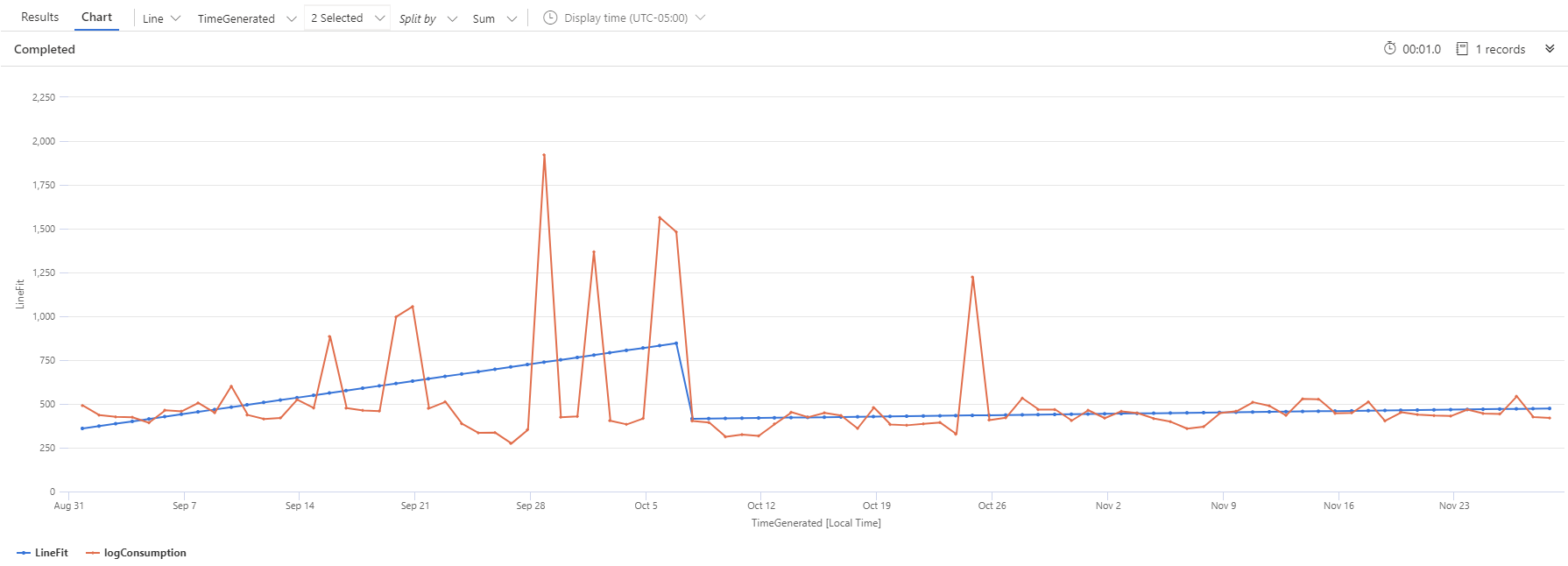
The series_fit_2lines() function splits the input array in two time series, determine the best split point index (SplitIDx), and calculate the best fit line for both, right and left series. The right side of the best fit line representing the current trend is used to calculate the estimated value of the log space usage 30 days in the future from current date:
//convert time range to scalar value
| extend numberOfDaysUsed = timeRange/1d
//using index of split point (days from the begining of the time series) calculate estimated log usage in 30 days from the current date
| extend estUsage = right_slope*(numberOfDaysUsed – SplitIDx + projectionDays) + right_interception
| project estUsage

Given the change in trend of the source data, the output value 508.017 MB of this script based on a two segments linear regression represents a better estimation.
Download script from GitHub
Final script:
//using series_fit_2lines() – useful when there is a sudden change in the data
let timeRange = 90d;
let projectionDays = 30;
Usage
| where TimeGenerated > ago(timeRange)
| make-series logConsumption = sum(Quantity) default = 0
on TimeGenerated in range (ago(timeRange) , ago(1d), 1d)
| extend (RSquare,SplitIDx,Variance, RVariance, LineFit, right_rsquare,right_slope,right_interception,right_variance,right_rvariance,left_rsquare,left_slope,left_variance,left_rvariance) = series_fit_2lines(logConsumption)
| extend numberOfDaysUsed = timeRange/1d
| render timechart
//using series_fit_2lines() – useful when there is a sudden change in the data
let timeRange = 90d;
let projectionDays = 30;
Usage
| where TimeGenerated > ago(timeRange)
| make-series logConsumption = sum(Quantity) default = 0
on TimeGenerated in range (ago(timeRange) , ago(1d), 1d)
//apply two segments linear regression to the logConsumption array to determine index of split, right slope, right nterception, LineFit
| extend (RSquare,SplitIDx,Variance, RVariance, LineFit, right_rsquare,right_slope,right_interception,right_variance,right_rvariance,left_rsquare,left_slope,left_variance,left_rvariance) = series_fit_2lines(logConsumption)
//convert time range to scalar value
| extend numberOfDaysUsed = timeRange/1d
//using index of split point (days from the begining of the time series) calculate estimated log usage in 30 days from the current date
| extend estUsage = right_slope*(numberOfDaysUsed – SplitIDx + projectionDays) + right_interception
| project estUsage
Often just an afterthought, log space consumption can potentially contribute to the cost of running solutions like Sentinel on top of the Azure Log Analytics platform and estimating future values can prove useful. Moreover, spikes and changes in the log usage trend are possibly indicators of unusual activity and subsequent analysis could also reveal or confirm the nature of the events that triggered those deviations.
The scripts can be converted to scheduled reports to run on weekly or monthly basis.